Shiny with PerformanceAnalytics Example

The folks at Rstudio have done some amazing work with the shiny package. From the shiny homepage, “Shiny makes it super simple for R users like you to turn analyses into interactive web applications that anyone can use.” Developing web applications has always appealed to me, but hosting, learning javascript, html, etc. made me put this pretty low on my priority list. With shiny, one can write web applications in R.

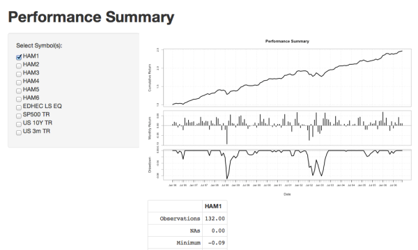
This example uses the managers dataset with calls to charts.PerformanceSummary and table.Stats from the PerformanceAnalytics package to display a plot and table in the shiny application.

Below is a screenshot of the application.
Screen Shot 2013-03-04 at 6.37.34 AM

You need to have shiny and Performance Analytics packages installed to run the application. Once those are installed, open your R prompt and run:

shiny::runGist("https://gist.github.com/rbresearch/5081906")

There is a great shiny tutorial from Rstudio as well as examples from SystematicInvestor for those interested in learning more.


Momentum in R: Part 4 with Quantstrat

The past few posts on momentum with R focused on a relatively simple way to backtest momentum strategies. In part 4, I use the quantstrat framework to backtest a momentum strategy. Using quantstrat opens the door to several features and options as well as an order book to check the trades at the completion of the backtest.

I introduce a few new functions that are used to prep the data and compute the ranks. I won’t go through them in detail, these functions are available in my github repo in the rank-functions folder.

This first chunk of code just loads the necessary libraries, data, and applies the ave3ROC function to rank the assets based on averaging the 2, 4, and 6 month returns. Note that you will need to load the functions in Rank.R and monthly-fun.R.

library(quantstrat)
library(PerformanceAnalytics)

currency("USD")
symbols <- c("XLY", "XLP", "XLE", "AGG", "IVV")
stock(symbols, currency="USD")

# get data for the symbols
getSymbols(symbols, from="2005-01-01", to="2012-12-31")

# create an xts object of monthly adjusted close prices
symbols.close <- monthlyPrices(symbols)

# create an xts object of the symbol ranks
sym.rank <- applyRank(x=symbols.close, rankFun=ave3ROC, n=c(2, 4, 6))

Created by Pretty R at inside-R.org

The next chunk of code is a critical step in preparing the data to be used in quantstrat. With the ranks computed, the next step is to bind the ranks to the actual market data to be used with quantstrat. It is also important to change the column names to e.g. XLY.Rank because that will be used as the trade signal column when quantstrat is used.

# this is an important step in naming the columns, e.g. XLY.Rank
# the "Rank" column is used as the trade signal (similar to an indicator)
# in the qstratRank function
colnames(sym.rank) <- gsub(".Adjusted", ".Rank", colnames(sym.rank))

# ensure the order of order symbols is equal to the order of columns 
# in symbols.close
stopifnot(all.equal(gsub(".Adjusted", "", colnames(symbols.close)), symbols))

# bind the rank column to the appropriate symbol market data
# loop through symbols, convert the data to monthly and cbind the data
# to the rank
for(i in 1:length(symbols)) {
  x <- get(symbols[i])
  x <- to.monthly(x,indexAt='lastof',drop.time=TRUE)
  indexFormat(x) <- '%Y-%m-%d'
  colnames(x) <- gsub("x",symbols[i],colnames(x))
  x <- cbind(x, sym.rank[,i])
  assign(symbols[i],x)
}

Created by Pretty R at inside-R.org

Now the backtest can be run. The function qstratRank is just a convenience function that hides the quantstrat implementation for my Rank strategy.

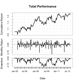
For this first backtest, I am trading the top 2 assets with a position size of 1000 units.

# run the backtest
bt <- qstratRank(symbols=symbols, init.equity=100000, top.N=2,
                  max.size=1000, max.levels=1)

# chart of returns
charts.PerformanceSummary(bt$returns[,"total"], geometric=FALSE, 
                          wealth.index=TRUE, main="Total Performance")

Created by Pretty R at inside-R.org

Rplot1

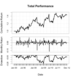
Changing the argument to max.levels=2 gives the flexibility of “scaling” in a trade. In this example, say asset ABC is ranked 1 in the first month — I buy 500 units. In month 2, asset ABC is still ranked 1 — I buy another 500 units.

# run the backtest
bt <- qstratRank(symbols=symbols, init.equity=100000, top.N=2,
                  max.size=1000, max.levels=2)

# chart of returns
charts.PerformanceSummary(bt$returns[,"total"], geometric=FALSE, 
                          wealth.index=TRUE, main="Total Performance")

Created by Pretty R at inside-R.org

Rplot2

Full code available here: quantstrat-rank-backtest.R

Momentum in R: Part 3

In the previous post, I demonstrated simple backtests for trading a number of assets ranked based on their 3, 6, 9, or 12 (i.e lookback periods) month simple returns. While it was not an exhaustive backtest, the results showed that when trading the top 8 ranked assets, the ranking based 3, 6, 9, and 12 month returns resulted in similar performance.

If the results were similar for the different lookback periods, which lookback period should I choose for my strategy? My answer is to include multiple lookback periods in the ranking method.

This can be accomplished by taking the average of the 6, 9, and 12 month returns, or any other n-month returns. This gives us the benefit of diversifying across multiple lookback periods. If I believe that the lookback period of 9 month returns is better than that of the 6 and 12 month, I can use a weighted average to give the 9 month return a higher weight so that it has more influence on determining the rank. This can be implemented easily with what I am calling the WeightAve3ROC() function shown below.

WeightAve3ROC <- function(x, n = c(1,3,6), weights = c(1/3, 1/3, 1/3)){
	# Computes the weighted average rate of change based on a vector of periods
	# and a vector of weights
	#
	# args:
	#   x = xts object of simple returns
	#   n = vector of periods to use n = (period1, period2, period3)
	#   weights = a vector of weights for computing the weighted average
	#
	# Returns:
	#   xts object of weighted average asset rate of change

  if((sum(weights) != 1) || (length(n) != 3) || (length(weights) != 3)){
    stop("The sum of the weights must equal 1 and the length of n and weights must be 3")
  } else{
    roc1 <- ROC(x, n = n[1], type = "discrete")
    roc2 <- ROC(x, n = n[2], type = "discrete")
    roc3 <- ROC(x, n = n[3], type = "discrete")
    wave <- (roc1 * weights[1] + roc2 * weights[2] + roc3 * weights[3]) / sum(weights)
    return(wave)
  }
}

Created by Pretty R at inside-R.org

The function is pretty self explanatory, but feel free to ask if you have any questions.

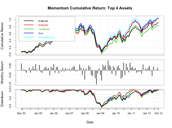
Now to the test results. The graph below shows the results from using 6, 9, and 12 month returns as well as an average of 6, 9, and 12 month returns and weighted average of 6, 9, and 12 month returns.

  • Case 1: simple momentum test based on 6 month ROC to rank
  • Case 2: simple momentum test based on 9 month ROC to rank
  • Case 3: simple momentum test based on 12 month ROC to rank
  • Case 4: simple momentum test based on average of 6, 9, and 12 month ROC to rank
  • Case 5: simple momentum test based on weighted average of 6, 9, and 12 month ROC to rank. Weights are 1/6, 2/3, 1/6 for 6, 9, and 12 month returns.

rbresearch

Here is a table of the returns and maximum drawdowns for the test.

4 Assets
        6-Month    9-Month    12-Month     Ave      Weighted Ave
 CAGR   0.07576607 0.08270242 0.07040551 0.08278835  0.08466842
 Max DD 0.4219671  0.4045444  0.4304139  0.4211499   0.3930215

This test demonstrates how it may be possible to achieve better risk adjusted returns (higher CAGR and lower drawdowns in this case) by considering multiple lookback periods in the ranking method.

Full R code is below. I have included all the functions in the R script below to make it easy for you to reproduce the tests and try things out, but I would recommend putting the functions in a separate file and using source() to load the functions to keep the code cleaner.

# rank_test2.R

# script to run a simple backtest comparing different ranking methods
# for a momentum based trading system

# remove objects from workspace
rm(list = ls())

# load required packages
library(FinancialInstrument)
library(TTR)
library(PerformanceAnalytics)

MonthlyAd <- function(x){
  # Converts daily data to monthly and returns only the monthly close 
  # Note: only used with Yahoo Finance data so far
  # Thanks to Joshua Ulrich for the Monthly Ad function
  # 
  # args:
  #   x = daily price data from Yahoo Finance
  #
  # Returns:
  #   xts object with the monthly adjusted close prices

  sym <- sub("\\..*$", "", names(x)[1])
  Ad(to.monthly(x, indexAt = 'lastof', drop.time = TRUE, name = sym))
}

CAGR <- function(x, m){
  # Function to compute the CAGR given simple returns
  #
  # args:
  #  x = xts of simple returns
  #  m = periods per year (i.e. monthly = 12, daily = 252)
  #
  # Returns the Compound Annual Growth Rate
  x <- na.omit(x)
  cagr <- apply(x, 2, function(x, m) prod(1 + x)^(1 / (length(x) / m)) - 1, m = m)
  return(cagr)
}

RankRB <- function(x){
  # Computes the rank of an xts object of ranking factors
  # ranking factors are the factors that are ranked (i.e. asset returns)
  #
  # args:
  #   x = xts object of ranking factors
  #
  # Returns:
  #   Returns an xts object with ranks
  #   (e.g. for ranking asset returns, the asset with the greatest return
  #    receives a  rank of 1)

  r <- as.xts(t(apply(-x, 1, rank, na.last = "keep")))
  return(r)
}

SimpleMomentumTest <- function(xts.ret, xts.rank, n = 1, ret.fill.na = 3){
  # returns a list containing a matrix of individual asset returns
  # and the comnbined returns
  # args:
  #  xts.ret = xts of one period returns
  #  xts.rank = xts of ranks
  #  n = number of top ranked assets to trade
  #  ret.fill.na = number of return periods to fill with NA
  #
  # Returns:
  #  returns an xts object of simple returns

  # trade the top n asset(s)
  # if the rank of last period is less than or equal to n,
  # then I would experience the return for this month.

  # lag the rank object by one period to avoid look ahead bias
  lag.rank <- lag(xts.rank, k = 1, na.pad = TRUE)
  n2 <- nrow(lag.rank[is.na(lag.rank[,1]) == TRUE])
  z <- max(n2, ret.fill.na)

  # for trading the top ranked asset, replace all ranks above n
  # with NA to set up for element wise multiplication to get
  # the realized returns
  lag.rank <- as.matrix(lag.rank)
  lag.rank[lag.rank > n] <- NA
  # set the element to 1 for assets ranked <= to rank
  lag.rank[lag.rank <= n] <- 1

  # element wise multiplication of the
  # 1 period return matrix and lagged rank matrix
  mat.ret <- as.matrix(xts.ret) * lag.rank

  # average the rows of the mat.ret to get the
  # return for that period
  vec.ret <- rowMeans(mat.ret, na.rm = TRUE)
  vec.ret[1:z] <- NA

  # convert to an xts object
  vec.ret <- xts(x = vec.ret, order.by = index(xts.ret))
  f <- list(mat = mat.ret, ret = vec.ret, rank = lag.rank)
  return(f)
}

WeightAve3ROC <- function(x, n = c(1,3,6), weights = c(1/3, 1/3, 1/3)){
  # Computes the weighted average rate of change based on a vector of periods
  # and a vector of weights
  #
  # args:
  #   x = xts object of simple returns
  #   n = vector of periods to use n = (period1, period2, period3)
  #   weights = a vector of weights for computing the weighted average
  #
  # Returns:
  #   xts object of weighted average asset rate of change

  if((sum(weights) != 1) || (length(n) != 3) || (length(weights) != 3)){
    stop("The sum of the weights must equal 1 and the length of n and weights must be 3")
  } else{
    roc1 <- ROC(x, n = n[1], type = "discrete")
    roc2 <- ROC(x, n = n[2], type = "discrete")
    roc3 <- ROC(x, n = n[3], type = "discrete")
    wave <- (roc1 * weights[1] + roc2 * weights[2] + roc3 * weights[3]) / sum(weights)
    return(wave)
  }
}

currency("USD")
symbols <- c("XLY", "XLP", "XLE", "XLF", "XLV", "XLI", "XLK", "XLB", "XLU", "EFA")
stock(symbols, currency = "USD", multiplier = 1)

# create new environment to store symbols
symEnv <- new.env()

# getSymbols and assign the symbols to the symEnv environment
getSymbols(symbols, from = '2002-09-01', to = '2012-10-20', env = symEnv)

# xts object of the monthly adjusted close prices
symbols.close <- do.call(merge, eapply(symEnv, MonthlyAd))

# monthly returns
monthly.returns <- ROC(x = symbols.close, n = 1, type = "discrete", na.pad = TRUE)

#############################################################################
# rate of change and rank based on a single period for 6, 9, and 12 months
#############################################################################

roc.six <- ROC(x = symbols.close , n = 6, type = "discrete")
rank.six <- RankRB(roc.six)

roc.nine <- ROC(x = symbols.close , n = 9, type = "discrete")
rank.nine <- RankRB(roc.nine)

roc.twelve <- ROC(x = symbols.close , n = 12, type = "discrete")
rank.twelve <- RankRB(roc.twelve)

#############################################################################
# rate of change and rank based on averaging 6, 9, and 12 month returns
#############################################################################
roc.ave <- WeightAve3ROC(x = symbols.close, n = c(6, 9, 12), 
                         weights = c(1/3, 1/3, 1/3))
rank.ave <- RankRB(roc.ave)

roc.weight.ave <- WeightAve3ROC(x = symbols.close, n = c(6, 9, 12), 
                                weights = c(1/6, 2/3, 1/6))
rank.weight.ave <- RankRB(roc.weight.ave)

#############################################################################
# run the backtest
#############################################################################

num.assets <- 4

# simple momentum test based on 6 month ROC to rank
case1 <- SimpleMomentumTest(xts.ret = monthly.returns, xts.rank = rank.six,
                            n = num.assets, ret.fill.na = 15)

# simple momentum test based on 9 month ROC to rank
case2 <- SimpleMomentumTest(xts.ret = monthly.returns, xts.rank = rank.nine,
                            n = num.assets, ret.fill.na = 15)

# simple momentum test based on 12 month ROC to rank
case3 <- SimpleMomentumTest(xts.ret = monthly.returns, xts.rank = rank.twelve,
                            n = num.assets, ret.fill.na = 15)

# simple momentum test based on average of 6, 9, and 12 month ROC to rank
case4 <- SimpleMomentumTest(xts.ret = monthly.returns, xts.rank = rank.ave,
                            n = num.assets, ret.fill.na = 15)

# simple momentum test based on weighted average of 6, 9, and 12 month ROC to rank
case5 <- SimpleMomentumTest(xts.ret = monthly.returns, xts.rank = rank.weight.ave,
                            n = num.assets, ret.fill.na = 15)

returns <- cbind(case1$ret, case2$ret, case3$ret, case4$ret, case5$ret)
colnames(returns) <- c("6-Month", "9-Month", "12-Month", "Ave", "Weighted Ave")

charts.PerformanceSummary(R = returns, Rf = 0, geometric = TRUE, 
                          main = "Momentum Cumulative Return: Top 4 Assets")

table.Stats(returns)

cagr <- CAGR(returns, m = 12)
max.dd <- maxDrawdown(returns)
print(cagr)
print(max.dd)

print("End")
Created by Pretty R at inside-R.org

Momentum in R: Part 2

Many of the sites I linked to in the previous post have articles or papers on momentum investing that investigate the typical ranking factors; 3, 6, 9, and 12 month returns. Most (not all) of the articles seek to find which is the “best” look-back period to rank the assets. Say that the outcome of the article is that the 6 month look-back has the highest returns. A trading a strategy that just uses a 6 month look-back period to rank the assets leaves me vulnerable to over-fitting based on the backtest results. The backtest tells us nothing more than which strategy performed the best in the past, it tells us nothing about the future… duh!

Whenever I review the results from backtests, I always ask myself a lot of “what if” questions. Here are 3 “what if” questions that I would ask for this backtest are:

  1. What if the strategy based on a 6 month look-back under performs and the 9 month or 3 month starts to over perform?
  2. What if the strategies based on 3, 6, and 9 month look-back periods have about the same return and risk profile, which strategy should I trade?
  3. What if the assets with high volatility are dominating the rankings and hence driving the returns?

The backtests shown are simple backtests meant to demonstrate the variability in returns based on look-back periods and number of assets traded.

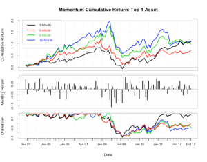
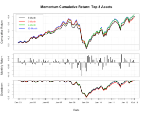
The graphs below show the performance of a momentum strategy using 3, 6, 9, and 12 month returns and trading the Top 1, 4, and 8 ranked assets. You will notice that there is significant volatility and variability in returns only trading 1 asset. The variability between look-back periods is reduced, but there is still no one clear “best” look-back period. There are periods of under performance and over performance for all look back periods in the test.

rbresearch

rbresearch

rbresearch


Here is the R code used for the backtests and the plots. Leave a comment if you have any questions about the code below.

library(FinancialInstrument)
library(TTR)
library(PerformanceAnalytics)

RankRB <- function(x){
  # Computes the rank of an xts object of ranking factors
  # ranking factors are the factors that are ranked (i.e. asset returns)
  #
  # args:
  #   x = xts object of ranking factors
  #
  # Returns:
  #   Returns an xts object with ranks
  #   (e.g. for ranking asset returns, the asset with the greatest return
  #    receives a  rank of 1)

  r <- as.xts(t(apply(-x, 1, rank, na.last = "keep")))
  return(r)
}

MonthlyAd <- function(x){
  # Converts daily data to monthly and returns only the monthly close 
  # Note: only used with Yahoo Finance data so far
  # Thanks to Joshua Ulrich for the Monthly Ad function
  # 
  # args:
  #   x = daily price data from Yahoo Finance
  #
  # Returns:
  #   xts object with the monthly adjusted close prices

  sym <- sub("\\..*$", "", names(x)[1])
  Ad(to.monthly(x, indexAt = 'lastof', drop.time = TRUE, name = sym))
}

CAGR <- function(x, m){
  # Function to compute the CAGR given simple returns
  #
  # args:
  #  x = xts of simple returns
  #  m = periods per year (i.e. monthly = 12, daily = 252)
  #
  # Returns the Compound Annual Growth Rate
  x <- na.omit(x)
  cagr <- apply(x, 2, function(x, m) prod(1 + x)^(1 / (length(x) / m)) - 1, m = m)
  return(cagr)
}

SimpleMomentumTest <- function(xts.ret, xts.rank, n = 1, ret.fill.na = 3){
  # returns a list containing a matrix of individual asset returns
  # and the comnbined returns
  # args:
  #  xts.ret = xts of one period returns
  #  xts.rank = xts of ranks
  #  n = number of top ranked assets to trade
  #  ret.fill.na = number of return periods to fill with NA
  #
  # Returns:
  #  returns an xts object of simple returns

  # trade the top n asset(s)
  # if the rank of last period is less than or equal to n,
  # then I would experience the return for this month.

  # lag the rank object by one period to avoid look ahead bias
  lag.rank <- lag(xts.rank, k = 1, na.pad = TRUE)
  n2 <- nrow(lag.rank[is.na(lag.rank[,1]) == TRUE])
  z <- max(n2, ret.fill.na)

  # for trading the top ranked asset, replace all ranks above n
  # with NA to set up for element wise multiplication to get
  # the realized returns
  lag.rank <- as.matrix(lag.rank)
  lag.rank[lag.rank > n] <- NA
  # set the element to 1 for assets ranked <= to rank
  lag.rank[lag.rank <= n] <- 1

  # element wise multiplication of the
  # 1 period return matrix and lagged rank matrix
  mat.ret <- as.matrix(xts.ret) * lag.rank

  # average the rows of the mat.ret to get the
  # return for that period
  vec.ret <- rowMeans(mat.ret, na.rm = TRUE)
  vec.ret[1:z] <- NA

  # convert to an xts object
  vec.ret <- xts(x = vec.ret, order.by = index(xts.ret))
  f <- list(mat = mat.ret, ret = vec.ret, rank = lag.rank)
  return(f)
}

currency("USD")
symbols <- c("XLY", "XLP", "XLE", "XLF", "XLV", "XLI", "XLK", "XLB", "XLU", "EFA")#, "TLT", "IEF", "SHY")
stock(symbols, currency = "USD", multiplier = 1)

# create new environment to store symbols
symEnv <- new.env()

# getSymbols and assign the symbols to the symEnv environment
getSymbols(symbols, from = '2002-09-01', to = '2012-10-20', env = symEnv)

# xts object of the monthly adjusted close prices
symbols.close <- do.call(merge, eapply(symEnv, MonthlyAd))

# monthly returns
monthly.returns <- ROC(x = symbols.close, n = 1, type = "discrete", na.pad = TRUE)

#############################################################################
# rate of change and rank based on a single period for 3, 6, 9, and 12 months
#############################################################################

roc.three <- ROC(x = symbols.close , n = 3, type = "discrete")
rank.three <- RankRB(roc.three)

roc.six <- ROC(x = symbols.close , n = 6, type = "discrete")
rank.six <- RankRB(roc.six)

roc.nine <- ROC(x = symbols.close , n = 9, type = "discrete")
rank.nine <- RankRB(roc.nine)

roc.twelve <- ROC(x = symbols.close , n = 12, type = "discrete")
rank.twelve <- RankRB(roc.twelve)

num.assets <- 4

# simple momentum test based on 3 month ROC to rank
case1 <- SimpleMomentumTest(xts.ret = monthly.returns, xts.rank = rank.three,
                            n = num.assets, ret.fill.na = 15)

# simple momentum test based on 6 month ROC to rank
case2 <- SimpleMomentumTest(xts.ret = monthly.returns, xts.rank = rank.six,
                            n = num.assets, ret.fill.na = 15)

# simple momentum test based on 9 month ROC to rank
case3 <- SimpleMomentumTest(xts.ret = monthly.returns, xts.rank = rank.nine,
                            n = num.assets, ret.fill.na = 15)

# simple momentum test based on 12 month ROC to rank
case4 <- SimpleMomentumTest(xts.ret = monthly.returns, xts.rank = rank.twelve,
                            n = num.assets, ret.fill.na = 15)

returns <- cbind(case1$ret, case2$ret, case3$ret, case4$ret)
colnames(returns) <- c("3-Month", "6-Month", "9-Month", "12-Month")

charts.PerformanceSummary(R = returns, Rf = 0, geometric = TRUE, 
                          main = "Momentum Cumulative Return: Top 4 Assets")

table.Stats(returns)

CAGR(returns, m = 12)

print("End")

Created by Pretty R at inside-R.org

Momentum with R: Part 1

Time really flies… it is hard to believe that it has been over a month since my last post. Work and life in general have consumed much of my time lately and left little time for research and blog posts. Anyway, on to the post!

This post will be the first in a series of to cover a momentum strategy using R.

One of my favorite strategies is a momentum or relative strength strategy. Here are just a few of the reasons why I like momentum:

  1. Simple to implement
  2. Long only or long/short portfolios
  3. Many ways to define the strength or momentum measure
  4. It just works

Also, a momentum strategy lends itself well to potential for diversification. The universe of instruments can be infinite, but the instruments traded are finite. Think about it this way… Investor A looks at 10 instruments and invests $1000 in the top 5 instruments ranked by momentum. Investor B looks at 100 instruments and invests $1000 in the top 5 instruments ranked by momentum. Investor A is limiting his potential for diversification by only having a universe of 10 instruments. Investor B has a much larger universe of instruments and can in theory be more diversified. Theoretically speaking, you can trade an infinite number of instruments with a finite amount of trading capital using a momentum or relative strength strategy.

Check out these links for further reading

In this first post of the series on momentum, I will go over some of the basic setup and functions we will be using.

The first step is to get data from yahoo.

require(quantstrat)

#Load ETFs from yahoo
currency("USD")
symbols = c("XLY", "XLP", "XLE", "XLF")
stock(symbols, currency="USD",multiplier=1)
getSymbols(symbols, src='yahoo', index.class=c("POSIXt","POSIXct"), from='2000-01-01')

#Convert to monthly and drop all columns except Adjusted Close
for(symbol in symbols) {
  x <- get(symbol)
  x <- to.monthly(x,indexAt='lastof',drop.time=TRUE)
  indexFormat(x) <- '%Y-%m-%d'
  colnames(x) <- gsub("x",symbol,colnames(x))
  x <- x[,6] #drops all columns except Adjusted Close which is 6th column
  assign(symbol,x)
}

Note that the for loop converts the data to monthly and subsets the data so that the only column we keep is the adjusted close column. We now have four objects (XLY, XLP, XLE, XLF) that have the Adjusted Close price.

> head(XLE)
           XLE.Adjusted
2000-01-31        22.89
2000-02-29        21.92
2000-03-31        24.56
2000-04-30        24.19
2000-05-31        27.04
2000-06-30        25.55

The next step is to merge these four objects into a single object holding the Adjusted Close price. We can do this in a simple one-liner in R!

#merge the symbols into a single object with just the close prices
symbols_close <- do.call(merge, lapply(symbols, get))
> head(symbols_close)
           XLY.Adjusted XLP.Adjusted XLE.Adjusted XLF.Adjusted
2000-01-31        24.06        18.36        22.89        18.09
2000-02-29        22.72        16.22        21.92        16.15
2000-03-31        25.89        16.77        24.56        19.04
2000-04-30        25.35        17.65        24.19        19.22
2000-05-31        23.98        18.92        27.04        19.65
2000-06-30        22.68        19.98        25.55        18.70

For the factor that will be ranked, I will use the 3 period rate of change (ROC).

#xts object of the 3 period ROC of each column in the close object
#The 3 period ROC will be used as the ranking factor
roc <- ROC(symbols_close, n = 3, type = "discrete")
> head(roc)
           XLY.Adjusted XLP.Adjusted XLE.Adjusted XLF.Adjusted
2000-01-31           NA           NA           NA           NA
2000-02-29           NA           NA           NA           NA
2000-03-31           NA           NA           NA           NA
2000-04-30   0.05361596  -0.03867102   0.05679336   0.06246545
2000-05-31   0.05545775   0.16646116   0.23357664   0.21671827
2000-06-30  -0.12398610   0.19141324   0.04030945  -0.01785714

Then we apply the rank function across each row of the roc object.

#xts object with ranks
#symbol with a rank of 1 has the highest ROC
r <- as.xts(t(apply(-roc, 1, rank)))


> head(r)
           XLY.Adjusted XLP.Adjusted XLE.Adjusted XLF.Adjusted
2000-01-31            1            2            3            4
2000-02-29            1            2            3            4
2000-03-31            1            2            3            4
2000-04-30            3            4            2            1
2000-05-31            4            3            1            2
2000-06-30            4            1            2            3

That will wrap up this first post for a quick and easy way to rank assets based on 3 month simple returns. Future posts will explore other methods for ranking and using quantstrat to backtest momentum.

Here is the code in full.

require(quantstrat)

#Load ETFs from yahoo
currency("USD")
symbols = c("XLY", "XLP", "XLE", "XLF")
stock(symbols, currency="USD",multiplier=1)
getSymbols(symbols, src='yahoo', index.class=c("POSIXt","POSIXct"), from='2000-01-01')

#Convert to monthly and drop all columns except Adjusted Close
for(symbol in symbols) {
  x <- get(symbol)
  x <- to.monthly(x,indexAt='lastof',drop.time=TRUE)
  indexFormat(x) <- '%Y-%m-%d'
  colnames(x) <- gsub("x",symbol,colnames(x))
  x <- x[,6] #drops all columns except Adjusted Close which is 6th column
  assign(symbol,x)
}

#merge the symbols into a single object with just the close prices
symbols_close <- do.call(merge, lapply(symbols, get))

#xts object of the 3 period ROC of each column in the close object
#The 3 period ROC will be used as the ranking factor
roc <- ROC(symbols_close, n = 3, type = "discrete")

#xts object with ranks
#symbol with a rank of 1 has the highest ROC
r <- as.xts(t(apply(-roc, 1, rank)))

Created by Pretty R at inside-R.org

“Computing for Data Analysis” with R on coursera

Just stumbled on across a course on coursera titled “Computing for Data Analysis” taught by Roger D. Peng the Johns Hopkins Bloomberg School of Public Health.

Here is the description of the course.

In this course you will learn how to program in R and how to use R for effective data analysis. You will learn how to install and configure software necessary for a statistical programming environment, discuss generic programming language concepts as they are implemented in a high-level statistical language. The course covers practical issues in statistical computing which includes programming in R, reading data into R, creating informative data graphics, accessing R packages, creating R packages with documentation, writing R functions, debugging, and organizing and commenting R code. Topics in statistical data analysis and optimization will provide working examples.

I just signed up for it! This course looks like a great opportunity to sharpen  skills in R and learn new things.

Alternative to Monte Carlo Testing

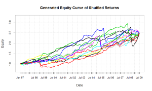
When we backtest a strategy on a portfolio, it is a simple analysis of a single period in time. There are ways to “stress test” a strategy such as monte carlo, random portfolios, or shuffling the returns in a random order. I could never really wrap my head around monte carlo and shuffling the returns seemed to be a better approach because the actual returns of the backtest are used, but it misses one important thing… the impact of consecutive periods of returns. If we are backtesting a strategy and we want to minimize max drawdown, consecutive down periods have a significant impact on max drawdown. If, for example, the max drawdown occured due to 4 consecutive months during 2008, we wan’t to keep those 4 months together when shuffling returns.

In my opinion, a better way to shuffle returns is to shuffle “blocks” of returns. This is nothing new, the TradingBlox software does monte carlo analysis this way. I had a look at the boot package and tseries package for their boot functions, but it was not giving me what I wanted. I wanted to visual a number of equity curves with blocks of returns randomly shuffled.

To accomplish this in R, I wrote two functions.  The shuffle_returns function takes an xts object of returns, the number of samples to run (i.e. how many equity curves to generate), and a number for how many periods of returns makes up a ‘block’ as arguments.The ran_gen function function is a function within the shuffle_returns function that is used to generate random blocks of returns.

shuffle_returns returns an xts object with the random blocks of returns so we can do further analysis such as max drawdown, plotting, or pretty much anything in the PerformanceAnalytics package that takes an xts object as an argument.

This is not a perfect implementation of this idea, so if anybody knows of a better way I’d be glad to hear from you.

The example below uses sample data from edhec and generates 100 equity curves with blocks of 5 consecutive period of returns.

R code:

require(PerformanceAnalytics)

#Function that grabs a random number and then repeats that number r times
ran_gen <- function(x, r){
  #x is an xts object of asset returns
  #r is for how many consecutive returns make up a 'block'
  vec <- c()
  total_length <- length(x)
  n <- total_length/r
  for(i in 1:n){
    vec <- append(vec,c(rep(sample(1:(n*100),1), r)))
  }
  diff <- as.integer(total_length - length(vec))
  vec <- append(vec, c(rep(sample(1:(n*100),1), len = diff)))
  return(vec)
}

shuffle_returns <- function(x, n, r){
  #x is an xts object of asset returns
  #n is the number of samples to run
  #r is for how many consecutive returns make up a 'block' and is passed to ran_gen

  mat <- matrix(data = x, nrow = length(x))
  for(i in 1:n){
    temp_random <- ran_gen(x = x, r = r)
    temp_mat <- as.matrix(cbind(x, temp_random))
    temp_mat <- temp_mat[order(temp_mat[,2]),]
    temp_ret_mat <- matrix(data = temp_mat[,1])
    mat <- cbind(mat, temp_ret_mat)
  }
  final_xts <- xts(mat, index(x))
  return(final_xts)
}

#get sample data
data(edhec)
a <- edhec[,1]
a <- head(a, -1)

start <- Sys.time()
yy <- shuffle_returns(a, 100, 5)
chart.CumReturns(yy[,1:NCOL(yy)], wealth.index = TRUE, ylab = "Equity", main ="Generated Equity Curve of Shuffled Returns")
end <- Sys.time()
print(end-start)

Created by Pretty R at inside-R.org

Strategy Diversification in R – follow up

The strategies used in Strategy Diversification in R were labeled as Strategy1 and Strategy2.

Strategy1

  • Indicator: 52 week Simple Moving Average
  • Entry Rule: Buy 1000 shares when price crosses and closes above 52 week Simple Moving Average
  • Exit Rule: Exit all positions when prices crosses and closes below 52 week Simple Moving Average
  • Classification: Long term trend following strategy

Strategy 2

  • Indicator: RSI(2) on weekly data
  • Entry Rule: Buy 100 shares when RSI(2) is less than 20 (Note that if RSI(2) is below 20 for N days, then you will have accumulated N * 100 shares)
  • Exit Rule: Exit all positions when RSI(2) is greater than 50
  • Classification: Short-Medium term reversal (dip buying) strategy

What did we diversify?

  1. Symbols? – No, the exact same instruments were used in the strategy.
  2. Markets? – No, see #1.
  3. Timeframe? Sort of, Strategy1 is a long term strategy and Strategy2 is a shorter term strategy, but both are on the weekly timeframe. We could diversify further by trading even shorter timeframes (i.e. Daily, Hourly, minute, tick, etc.)
  4. Strategy? Yes, Strategy1 is a trend following strategy and Strategy2 is a reversal strategy.
  5. Risk Levels? Yes, Strategy2 trades more often, but in smaller increments.

We achieved fairly low correlations by achieving only three “levels” of diversification. Think what we could do by using a “kitchen sink” portfolio with grains, softs, metals, currencies, stocks, fixed income, international stocks, international fixed income, style ETFs, etc.

Three R script files were used in the last post.

strategy1.R, strategy2.R, and correlation chart.R

The R scripts are pretty self explanatory so I won’t go into much detail. However, I do want to call attention to 2 lines of code from strategy1.R. The code for strategy2.R is virtually identical.

# logarithmic returns of the equity curve of strategy1.
strategy1_eclogret <- ec$logret

# write the logarithmic returns of strategy 1 to a csv file with the filename "strategy1.csv"
# you will have to change the file where you want to save it
write.zoo(strategy1_eclogret, file = "~/R/strats_for_cor/strategy1.csv", sep=",")

Created by Pretty R at inside-R.org

Here is the code to make the correlation chart.

#Load the packages used
require(PerformanceAnalytics)

# load the strategy 1 returns
strat1 <- as.xts(read.zoo(file = "~/R/strats_for_cor/strategy1.csv", header = TRUE, sep=","))
colnames(strat1) <- "strat1"

# load the strategy 2 returns
strat2 <- as.xts(read.zoo(file = "~/R/strats_for_cor/strategy2.csv", header = TRUE, sep=","))
colnames(strat2) <- "strat2"

suppressWarnings(chart.RollingCorrelation(strat1, strat2, width = 52, xaxis = TRUE, 
                                          colorset = rich8equal, legend.loc = "bottomright",
                                          main = "Rolling 52 Week Correlation"))

Created by Pretty R at inside-R.org

And that is all there is to it. (run strategy1.R, run strategy2.R, then run correlation chart.R – don’t forget to change the file directory!)

I listed 5 “levels” or ways to achieve diversification… what are other ways we can diversify? – post your ideas in the comments

Strategy Diversification in R

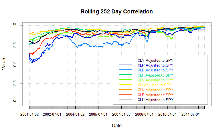
In my last post, I looked at the correlations of different instruments. Understanding the correlations of instruments is important when developing a strategy and selecting the assets to include. In theory, selecting highly correlated instruments for a portfolio or strategy will be more volatile than a portfolio or strategy with several uncorrelated instruments. This sounds great in theory, but can be difficult to apply in real life. Why? – correlations change over time and just diversifying among instruments is not enough. Just take a look at the graph below from my post on correlations as well as Systematic Investor’s analysis of Cross Sectional Correlation.

Correlations are changing over time and markets are becoming more correlated in recent times. As the correlations between markets and instruments increases, the impact of diversification decreases. You may be asking yourself (like I am), “If I can’t diversify among assets, what else can I do to diversify?” My answer to this is to diversify in as many ways as you can – trade multiple strategies, multiple timeframes, multiple risk levels, multiple markets, multiple instruments, etc.

To demonstrate this, I will take two strategies:

  • Strategy1 – longer term strategy
  • Strategy2 – shorter term strategy

(Yes… I realize that I am being very vague about the strategies at this point, more on the strategy details later in the post.)

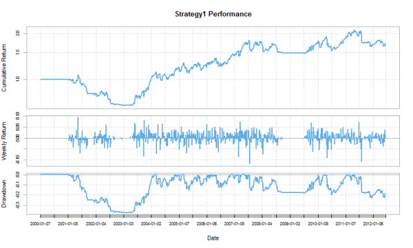
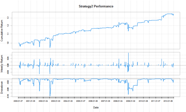
Here are the outcomes of each strategy using quantstrat to backtest.

Strategy 1

CAGR maxDD MAR
6.599 -36.358 0.182

rbresearch

Strategy 2

CAGR maxDD MAR
2.637 -9.637 0.274

rbresearch

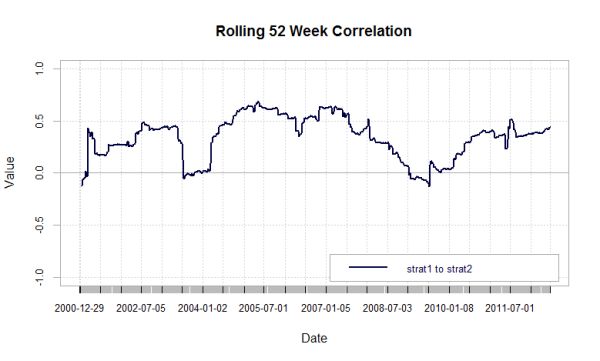
How does each strategy correlate to eachother?

rbresearch

The chart above shows that Strategy 1 is not very strongly correlated with Strategy 2.

Now for more information on the strategies.

  • Strategy 1 and Strategy 2 both trade the same universe of instruments (“XLY”, “XLP”, “XLE”, “XLF”, “XLV”, “XLI”, “XLK”, “XLB”, “XLU”)
  • Strategy 1 is a 52 week moving average strategy and trades 1000 contracts per trade*
  • Strategy 2 is a RSI(2) on weekly data strategy and trades 100 contracts per trade*
  • *Note on position sizing. Normally I would do a volatility based position sizing, but the RSI(2) strategy took about 20 minutes to complete the test because of the looping in the order sizing function. So for brevity and testing purposes I used fixed contract sizes as stated above for each strategy.

Are you surprised that two strategies that trade the exact same set of instruments would not have a higher correlation? I was!

This example reinforces how diversification can be achieved in more ways than one.

In follow-up posts, I will share the R code for the strategies and show how I plotted the correlations.